Direct Python usage

Minimal example calling IMRPhenomTHM without external waveform interfaces.

%matplotlib inline

import matplotlib.pyplot as plt
import numpy as np
import phenomxpy

kwargs = dict(
    eta=0.2,
    total_mass=40.0,
    s1=[0.4, 0.1, 0.5],
    s2=[0.3, 0.2, -0.3],
    f_min=20.0,
    delta_t=1.0 / 4096,
    distance=100.0,
    inclination=np.pi / 3,
)

phen = phenomxpy.IMRPhenomTPHM(**kwargs)
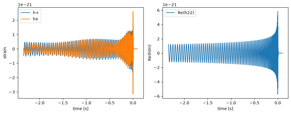
hp, hc, times = phen.compute_polarizations(times=None)
hlms, times = phen.compute_CPmodes(times=None)

fig, axs = plt.subplots(1, 2, figsize=(10, 4))

axs[0].plot(times, hp, label="h+")
axs[0].plot(times, hc, label="hx")
axs[0].set_xlabel("time [s]")
axs[0].set_ylabel("strain")
axs[0].legend()

axs[1].plot(times, np.real(hlms["22"]), label="Re(h22)")
axs[1].set_xlabel("time [s]")
axs[1].set_ylabel("Re(hlm)")
axs[1].legend()

plt.tight_layout()
plt.show()

Custom time array

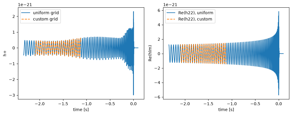
custom_times = times[1000:5000]
hp_custom, hc_custom, custom_times = phen.compute_polarizations(times=custom_times)
hlms_custom, custom_times = phen.compute_CPmodes(times=custom_times)

select = np.arange(1000, 5000)
hc_uniform_common = hc[select]
hc_diff = np.abs(hc_uniform_common - hc_custom)

fig, axs = plt.subplots(1, 2, figsize=(10, 4))

axs[0].plot(times, hp, label="uniform grid")
axs[0].plot(custom_times, hp_custom, "--", label="custom grid")
axs[0].set_xlabel("time [s]")
axs[0].set_ylabel("h+")
axs[0].legend()

axs[1].plot(custom_times, hc_diff)
axs[1].set_xlabel("time [s]")
axs[1].set_ylabel("|hx_uniform - hx_custom|")

plt.tight_layout()
plt.show()

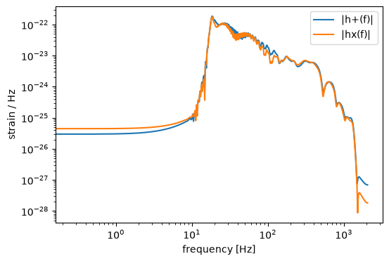
Fourier-domain polarizations

phen = phenomxpy.IMRPhenomTPHM(**kwargs, delta_f=0, condition=True)
hpf, hcf, frequencies = phen.compute_fd_polarizations()

fig, ax = plt.subplots(figsize=(6, 4))
ax.loglog(frequencies, np.abs(hpf), label="|h+(f)|")
ax.loglog(frequencies, np.abs(hcf), label="|hx(f)|")
ax.set_xlabel("frequency [Hz]")
ax.set_ylabel("strain / Hz")
ax.legend()
plt.show()